Multiple maps using subplots

import ee
import cartoee as cee
import cartopy.crs as ccrs

%pylab inline

Populating the interactive namespace from numpy and matplotlib

ee.Initialize()

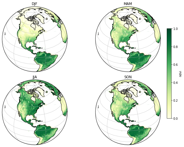
Seasonal NDVI example

In this example we will compute the seasonal average NDVI values for the globe and plot the four seasons on the same figure.

# function to add NDVI band to imagery
def calc_ndvi(img):
    ndvi = img.normalizedDifference(['Nadir_Reflectance_Band2','Nadir_Reflectance_Band1'])
    return img.addBands(ndvi.rename('ndvi'))

# MODIS Nadir BRDF-Adjusted Reflectance with NDVI band
modis = ee.ImageCollection('MODIS/006/MCD43A4')\
        .filterDate('2010-01-01','2016-01-01')\
        .map(calc_ndvi)

# set parameters for plotting
ndviVis = {'min':0,'max':1,'bands':'ndvi'}
bbox = [-180,-60,180,90]

# get land mass feature collection
land = ee.FeatureCollection('USDOS/LSIB_SIMPLE/2017')

# calculate seasonal averages and clip to land features
djf = modis.filter(ee.Filter.calendarRange(12,3,'month')).mean().clip(land)
mam = modis.filter(ee.Filter.calendarRange(3,6,'month')).mean().clip(land)
jja = modis.filter(ee.Filter.calendarRange(6,9,'month')).mean().clip(land)
son = modis.filter(ee.Filter.calendarRange(9,12,'month')).mean().clip(land)

# set up a blank map with multiple subplots
fig,ax = plt.subplots(ncols=2,nrows=2,figsize=(10,7),
                      subplot_kw={'projection': ccrs.Orthographic(-80,35)})

# format images and subplot titles with same dimensions as subplots
imgs = np.array([[djf,mam],[jja,son]])
titles = np.array([['DJF','MAM'],['JJA','SON']])

for i in range(len(imgs)):
    for j in range(len(imgs[i])):
        ax[i,j] = cee.addLayer(imgs[i,j],ax=ax[i,j],
                               region=bbox,dims=500,
                               visParams=ndviVis,cmap='YlGn'
                              )
        ax[i,j].coastlines()
        ax[i,j].gridlines(linestyle='--')
        ax[i,j].set_title(titles[i,j])

plt.tight_layout()

cax = fig.add_axes([0.9, 0.2, 0.02, 0.6])
cb = cee.addColorbar(ax[i,j],cax=cax,cmap='YlGn',visParams=ndviVis)

plt.show()

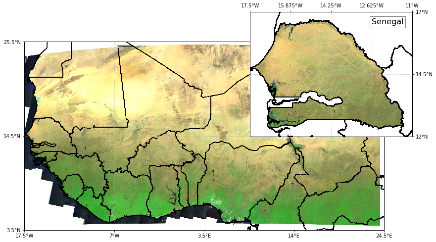
Map inset example

In this example we are going to take a regional image from EE, plot the entire region, and plot a smaller country within the region as a subset. This specific example will create a map for West Africa showing a Landsat mosaic and create an inset map of Senegal using the same Landsat mosaic.

# get a country FeatureCollection
countries = ee.FeatureCollection('USDOS/LSIB_SIMPLE/2017')
# filter the countries for a specific county
country = 'Senegal'
senegal = ee.Feature(countries.filter(ee.Filter.eq('country_na',country)).first())
# create an ee.Image from a FeatureCollection
adminImg = ee.Image().paint(countries,color='#000000',width=4)

# get a Landsat mosaic for West Africa
waLandsat = ee.Image('projects/servir-wa/regional_west_africa/Landsat_SR/Landsat_SR_prewet_2012_2014')
# specify the visualization parameters
lsVis = {'min':50,'max':5500,'gamma':1.5,'bands':'swir2,nir,green'}

# import some styling functions
from cartopy.mpl.gridliner import LATITUDE_FORMATTER, LONGITUDE_FORMATTER

# setup blank figure
fig = plt.figure(figsize=(15,7))

# region for the main map
mainBox = [-17.5,3.5,24.5,25.5]

# set blank map for the main plot and add layers
ax_main = fig.add_subplot(1, 1, 1,projection=ccrs.PlateCarree())
ax_main = cee.addLayer(waLandsat,visParams=lsVis,region=mainBox,dims=2500,ax=ax_main)
ax_main = cee.addLayer(adminImg,region=mainBox,dims=1500,ax=ax_main)

# main map styling
xmain = np.linspace(-17.5,24.5,5)
ymain = np.linspace(3.5,25.5,3)
ax_main.gridlines(xlocs=xmain, ylocs=ymain,linestyle=':')
# set custom formatting for the tick labels
ax_main.xaxis.set_major_formatter(LONGITUDE_FORMATTER)
ax_main.yaxis.set_major_formatter(LATITUDE_FORMATTER)
# set tick labels
ax_main.set_xticks(xmain, crs=ccrs.PlateCarree())
ax_main.set_yticks(ymain, crs=ccrs.PlateCarree())


# region for the map inset
insetBox = [-17.5,12,-11,17]

# setup inset map and add layers
ax_inset = fig.add_axes([0.45, 0.5, 0.6, 0.5],projection=ccrs.PlateCarree())
ax_inset = cee.addLayer(waLandsat.clip(senegal),visParams=lsVis,region=insetBox,dims=2500,ax=ax_inset)
ax_inset = cee.addLayer(adminImg,region=insetBox,ax=ax_inset)

# inset map styling
xinset = np.linspace(-17.5,-11,5)
yinset = np.linspace(12,17,3)
ax_inset.gridlines(xlocs=xinset, ylocs=yinset,linestyle=':')
# set custom formatting for the tick labels
ax_inset.xaxis.set_major_formatter(LONGITUDE_FORMATTER)
ax_inset.yaxis.set_major_formatter(LATITUDE_FORMATTER)
ax_inset.xaxis.tick_top()
ax_inset.yaxis.tick_right()
# set inset tick labels
ax_inset.set_xticks(xinset, crs=ccrs.PlateCarree())
ax_inset.set_yticks(yinset, crs=ccrs.PlateCarree())

# add some text to the inset as a pseudo-title
ax_inset.text(-12.63,16.5,country,fontsize=16,bbox=dict(facecolor='white', alpha=0.5,edgecolor='k'))

plt.show()